Titanic Machine Learning from Disaster
Based on the Titanic Competition on Kaggle Kaggle Competition: Titanic Machine Learning from Disaster
by Curtis Gibeom Kim
March 2017
1. Introduction
1.1 Goal
It is your job to predict if a passenger suvived the sinking of the Titanic or not. For each Passengerld in the test set, you must predict a 0 or 1 value for the survived variable. More Inforamation: Kaggle Competition: Titanic Machine Learning from Disaster
1.2 Dataset
- Training set + feature engineering
- Test set
1.3 Data Dictionary
- Survived: Survived or Not
- Pclass: Ticket class(1st = Upper, 2nd = Middle, 3rd = Lower)
- Sex: Sex(Male or Female)
- Age: Age in years
- SibSp: the number of siblings and spouses aboard the Titanic (Sibling and Spouse)
- Parch: the number of parents and children aboard the Titanic (Parent and Child)
- Ticket: Ticket number
- Fare: Passenger fare
- Cabin: Cabin number
-
Embarked: Port of Embarkation
- 1 = 1st, 2 = 2nd, 3 = 3rd
- 0 = No, 1 = Yes
-
C = Cherbourg, Q = Queenstown, S = Southampton
- Continuous variables: Age, Fare
- Categorical variables: Pclass, Sex, Cabin, Embarked, SibSp and Parch
1.4 Import libraries
import numpy as np
import pandas as pd
import string
import seaborn as sns
from sklearn import preprocessing
from sklearn.preprocessing import OneHotEncoder
## Model
from sklearn.linear_model import LogisticRegression
from sklearn.svm import SVC, LinearSVC
from sklearn.ensemble import RandomForestClassifier, ExtraTreesClassifier
from sklearn.naive_bayes import GaussianNB
## Evaluation
from sklearn.model_selection import train_test_split
from sklearn.model_selection import cross_val_score
2. Understand dataset
2.1 Data load and Descriptive statistics
To begin with, we need to understand titanic dataset. There are two types of dataset, the first one is train dataset which has 891 observations of 12 variables and the second one is test data has 418 observations of 11 variables. Also it should be needed to check missing values in obsevations
df_original = pd.read_csv('train.csv')
df_test = pd.read_csv('test.csv')
df_original.shape
(891, 12)
df_test.shape
(418, 11)
df_original.info()
<class 'pandas.core.frame.DataFrame'>
RangeIndex: 891 entries, 0 to 890
Data columns (total 12 columns):
PassengerId    891 non-null int64
Survived       891 non-null int64
Pclass         891 non-null int64
Name           891 non-null object
Sex            891 non-null object
Age            714 non-null float64
SibSp          891 non-null int64
Parch          891 non-null int64
Ticket         891 non-null object
Fare           891 non-null float64
Cabin          204 non-null object
Embarked       889 non-null object
dtypes: float64(2), int64(5), object(5)
memory usage: 83.6+ KB
df_original.describe()
| PassengerId | Survived | Pclass | Age | SibSp | Parch | Fare | |
|---|---|---|---|---|---|---|---|
| count | 891.000000 | 891.000000 | 891.000000 | 714.000000 | 891.000000 | 891.000000 | 891.000000 |
| mean | 446.000000 | 0.383838 | 2.308642 | 29.699118 | 0.523008 | 0.381594 | 32.204208 |
| std | 257.353842 | 0.486592 | 0.836071 | 14.526497 | 1.102743 | 0.806057 | 49.693429 |
| min | 1.000000 | 0.000000 | 1.000000 | 0.420000 | 0.000000 | 0.000000 | 0.000000 |
| 25% | 223.500000 | 0.000000 | 2.000000 | 20.125000 | 0.000000 | 0.000000 | 7.910400 |
| 50% | 446.000000 | 0.000000 | 3.000000 | 28.000000 | 0.000000 | 0.000000 | 14.454200 |
| 75% | 668.500000 | 1.000000 | 3.000000 | 38.000000 | 1.000000 | 0.000000 | 31.000000 |
| max | 891.000000 | 1.000000 | 3.000000 | 80.000000 | 8.000000 | 6.000000 | 512.329200 |
df_original.isnull().sum()
PassengerId      0
Survived         0
Pclass           0
Name             0
Sex              0
Age            177
SibSp            0
Parch            0
Ticket           0
Fare             0
Cabin          687
Embarked         2
dtype: int64
df_test.isnull().sum()
PassengerId      0
Pclass           0
Name             0
Sex              0
Age             86
SibSp            0
Parch            0
Ticket           0
Fare             1
Cabin          327
Embarked         0
dtype: int64
2.2 Drop unnecessary variables
df_original = df_original.drop(['PassengerId', "Name", "Ticket"], axis = 1)
df_test = df_test.drop(["Name", "Ticket"], axis = 1)
2.3 Imputing missing values
We need to fill missing values with mean, median, or mode values.
-
Missing value list: Age, Embarked, Cabin, Fare
- Age will be filled with mean values
- Embarked will be filled with mode values
- Cabin will be filled with Null
- Fare will be filled with median values
#Training Dataset
df_original.Age = df_original.Age.fillna(np.mean(df_original.Age))
df_original.Embarked = df_original.Embarked.fillna(df_original.Embarked.mode()[0][0])
df_original.Cabin = df_original.Cabin.fillna("Unknown")
#Test Dataset
df_test.Age = df_test.Age.fillna(np.mean(df_test.Age))
df_test.Cabin = df_test.Cabin.fillna("Unknown")
df_test.Fare = df_test.Fare.fillna(df_test["Fare"].median())
2.4 Converting Age and Fare data to intager
As in the descriptive statistics, minimum of “Age” is 0.42, so we need to convert float data type into int data type.
# Training Data
df_original.Fare = df_original.Fare.astype(int)
df_original.Age = df_original.Age.astype(int)
# Test Data
df_test.Fare = df_test.Fare.astype(int)
df_test.Age = df_test.Age.astype(int)
3. Visualization
3.1 Continuous variables
3.1.1 “Age” and “Fare”
sns.set(style = "white", palette = 'muted', color_codes = True)
fig, ax = plt.subplots(1,2, figsize=(12,7), sharex = True)
sns.despine(left=True)

sns.distplot(df_original['Age'],kde = True, color = 'y', ax=ax[0])
sns.distplot(df_original['Fare'], bins=20, kde = True, color = 'g', ax=ax[1])
<matplotlib.axes._subplots.AxesSubplot at 0x7f2b4affe750>
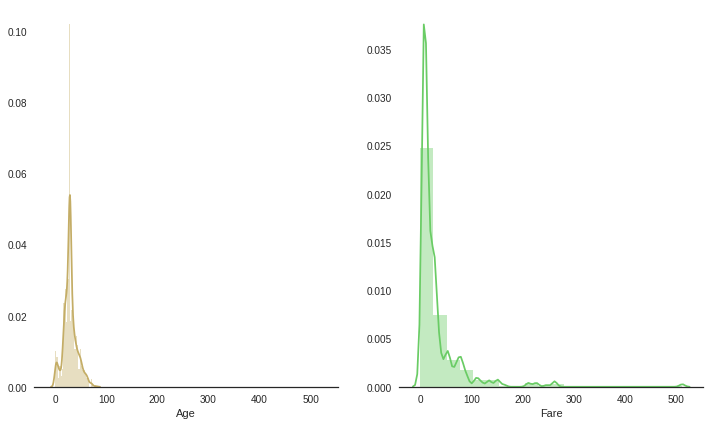
“Age” and “Fare” are needed to do feature scaling
# Training dataset
o_standard_scale = preprocessing.StandardScaler().fit(df_original[["Age", "Fare"]])
df_original_std_Age_Fare=o_standard_scale.transform(df_original[["Age", "Fare"]])
# Test dataset
t_standard_scale = preprocessing.StandardScaler().fit(df_test[["Age", "Fare"]])
df_test_std_Age_Fare=t_standard_scale.transform(df_test[["Age", "Fare"]])
3.2 Categorical variables
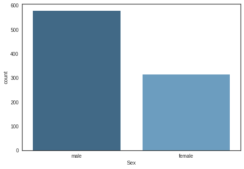
3.2.1 “Sex”
sns.countplot(x="Sex", data=df_original, palette="Blues_d")
<matplotlib.axes._subplots.AxesSubplot at 0x7f2b503b2350>
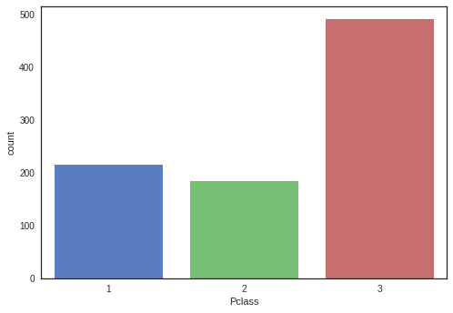
3.2.2 “Pclass”
[1, 2, 3], the values have no meaning of their own number. They are needed to comvert dummies values.
sns.countplot(x="Pclass", data=df_original)
<matplotlib.axes._subplots.AxesSubplot at 0x7f2b50180d50>
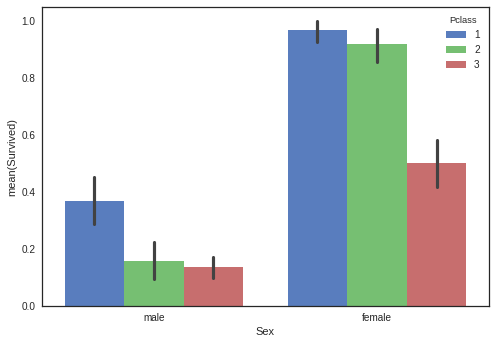
#Pclass, Sex, Cabin, Embarked, Sibsp/Parch
sns.barplot(x='Sex', y='Survived', hue='Pclass', data=df_original)
<matplotlib.axes._subplots.AxesSubplot at 0x7f2b50101bd0>
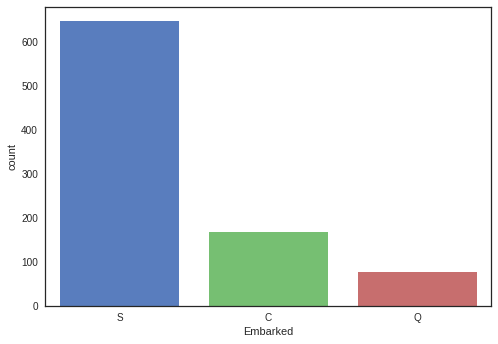
3.2.3 “Embarked”
sns.countplot(x="Embarked", data=df_original)
<matplotlib.axes._subplots.AxesSubplot at 0x7f2b500d0d50>
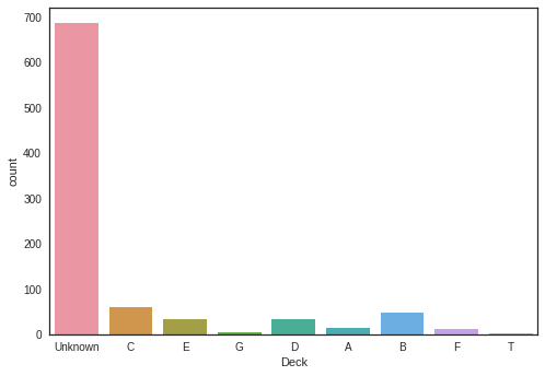
3.2.4 “Cabin”
“Cabin” values are needed to be groupped by their upper group like deck “C”, “D”.
def substrings_in_string(big_string, substrings):
    for s in substrings:
        if string.find(big_string, s) != -1: ## if not found return -1
            return s
    return np.nan
# Training data
df_original.Cabin = df_original.Cabin.fillna("Unknown")
cabin_list = ['A', 'B', 'C', 'D', 'E', 'F', 'T', 'G', 'Unknown']
df_original['Deck']=df_original['Cabin'].map(lambda x: substrings_in_string(x, cabin_list))
sns.countplot(x='Deck', data=df_original)
df_original = df_original.drop(['Cabin'], axis = 1)
# Test data
df_test.Cabin = df_test.Cabin.fillna("Unknown")
df_test['Deck']=df_test['Cabin'].map(lambda x: substrings_in_string(x, cabin_list))
df_test = df_test.drop(['Cabin'], axis = 1)
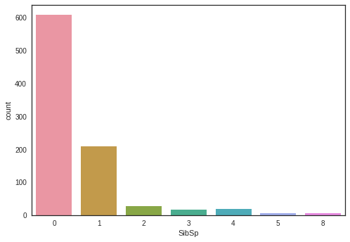
3.2.5 “SibSp”
sns.countplot(x='SibSp', data=df_original)
<matplotlib.axes._subplots.AxesSubplot at 0x7f2b502e1f10>
3.2.6 “Parch”
sns.countplot(x='Parch', data=df_original)
<matplotlib.axes._subplots.AxesSubplot at 0x7f2b507b0450>
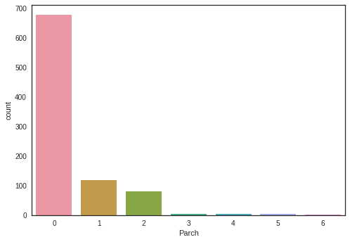
We might need to combine SibSp and Parch into Faimly_Size
# Training data
df_original['Family_Size'] = df_original['SibSp'] + df_original['Parch']
# Test data
df_test['Family_Size'] = df_test['SibSp'] + df_test['Parch']
3.3 Convert categorical variables into numeric
# Training data
# Male : 1 Female : 0
temp_sex_col = df_original["Sex"]
df_original.ix[:, "Sex"] = preprocessing.LabelEncoder().fit_transform(df_original["Sex"])
## np.newaxis is to increase the dimension
#OneHotEncoder.fit_transform()(matrix) : <891x3 sparse matrix of type '<type 'numpy.float64'>'with 891 stored elements in Compressed Sparse Row format>
#891X3 sparse matrix.toarray():[0,1,0], 2:[1, 0, 0] [0,0,1] form
dfX2 = pd.DataFrame(OneHotEncoder().fit_transform(df_original["Pclass"].as_matrix()[:,np.newaxis]).toarray(),
                    columns=['first_class', 'second_class', 'third_class'], index=df_original.index)
df_original = pd.concat([df_original, dfX2], axis=1)
del(df_original["Pclass"])
# Embarked
df_original.ix[:, "Embarked"] = preprocessing.LabelEncoder().fit_transform(df_original["Embarked"])

# Test data
temp_sex_col_t = df_test["Sex"]
df_test.ix[:, "Sex"] = preprocessing.LabelEncoder().fit_transform(df_test["Sex"])
dfX2_t = pd.DataFrame(OneHotEncoder().fit_transform(df_test["Pclass"].as_matrix()[:,np.newaxis]).toarray(),
                 columns=['first_class', 'second_class', 'third_class'], index=df_test.index)
df_test = pd.concat([df_test, dfX2_t], axis=1)
del(df_test["Pclass"])
df_test.ix[:, "Embarked"] = preprocessing.LabelEncoder().fit_transform(df_test["Embarked"])
#['A', 'B', 'C', 'D', 'E', 'F', 'G', 'T', 'Unknown'] [1,2, 3, 4, 5, 6, 7, 8]
# Training data
df_original.ix[:, "Deck"] = preprocessing.LabelEncoder().fit_transform(df_original["Deck"])
# Test data
df_test.ix[:, "Deck"] = preprocessing.LabelEncoder().fit_transform(df_test["Deck"])
3.4 Correlation of features
corr = df_original.corr()
fig, ax = plt.subplots(figsize=(20,20))
sns.heatmap(corr, vmax=1, square = True, annot = True, fmt='.4g', ax = ax)
<matplotlib.axes._subplots.AxesSubplot at 0x7f2b4bd8f290>
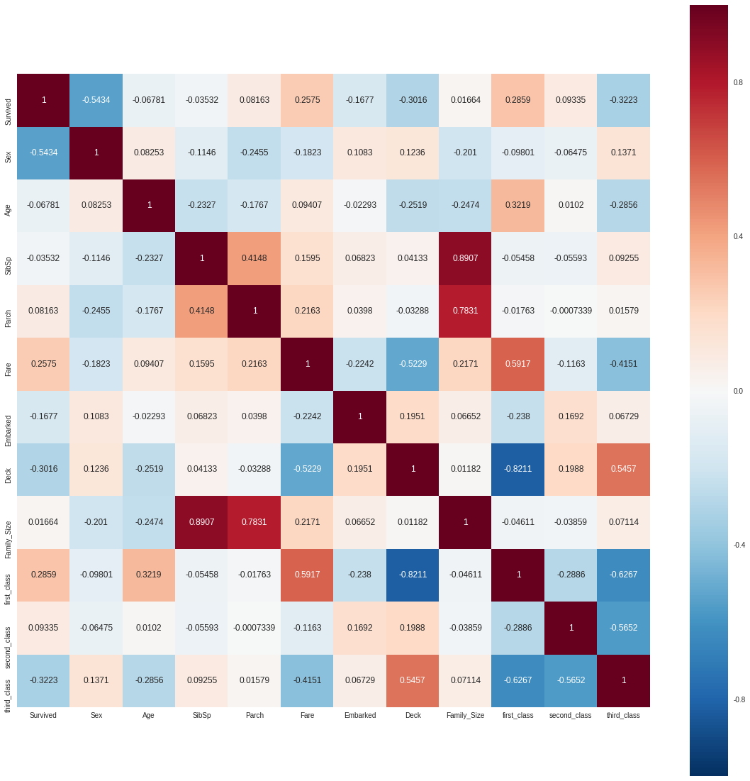
df_original.corr()['Survived']
Survived        1.000000
Sex            -0.543351
Age            -0.067809
SibSp          -0.035322
Parch           0.081629
Fare            0.257482
Embarked       -0.167675
Deck           -0.301570
Family_Size     0.016639
first_class     0.285904
second_class    0.093349
third_class    -0.322308
Name: Survived, dtype: float64
3.4.1 Feature cleaning
- delete “SibSp” and “Parch”
- Sex will be divided by three features including “Child”
### Modify : drop "SibSp", "Parch"
# Training data
df_original = df_original.drop(['SibSp', "Parch"], axis = 1)
# Test data
df_test = df_test.drop(['SibSp', "Parch"], axis = 1)
# average survived passengers by age
f, ax = plt.subplots(1,1,figsize=(40,10))
average_age = df_original[["Age", "Survived"]].groupby(['Age'],as_index=False).mean()
sns.barplot(x='Age', y='Survived',color = 'g', data=average_age)
<matplotlib.axes._subplots.AxesSubplot at 0x7f2b4bd30c90>
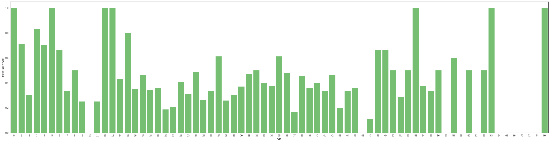
Age < 16 looks like high chances for surviva, so new feature is necessary
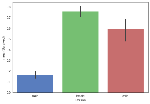
### Age < 16 looks like high chances for survival
def get_person(passenger):
    age, sex = passenger
    return 'child' if age < 16 else sex
# Training data
del(df_original['Sex'])
df_original = pd.concat([df_original, temp_sex_col], axis=1)
df_original['Person'] = df_original[['Age', "Sex"]].apply(get_person, axis=1)
df_original = df_original.drop(['Sex'], axis = 1)
# 1: Male, 0: Female, 2: Child
sns.barplot(x='Person', y="Survived", data = df_original, order=["male","female","child"])

# Test data
del(df_test["Sex"])
df_test = pd.concat([df_test, temp_sex_col_t], axis=1)
df_test["Person"] = df_test[["Age", "Sex"]].apply(get_person, axis=1)
df_test = df_test.drop(["Sex"], axis=1)
# Person dummies variables
# Training data
person_dummies_origin = pd.get_dummies(df_original["Person"])
person_dummies_origin.columns = ["Child", "Female", "Male"]
### drop Male because it has seldomly affect survived passengers
person_dummies_origin.drop(["Male"], axis = 1, inplace=True)
df_original = df_original.join(person_dummies_origin)

# Test data
person_dummies_test = pd.get_dummies(df_test["Person"])
person_dummies_test.columns = ["Child", "Female", "Male"]
person_dummies_test.drop(["Male"], axis = 1, inplace=True)
df_test = df_test.join(person_dummies_test)
Male might be needed to delete, because it has sedomly affect survived rate.
# Training data
df_original.drop(["Person"], axis=1, inplace = True)
# Test data
df_test.drop(["Person"], axis=1, inplace = True)
### drop third class
# Training data
df_original.drop(["third_class"], axis=1, inplace = True)
# Test data
df_test.drop(["third_class"], axis=1, inplace = True)
4. Final Dataset
# Training data
df_original[["Age", "Fare"]] = df_original_std_Age_Fare
# Test data
df_test[["Age", "Fare"]] = df_test_std_Age_Fare
df_original.tail()
| Survived | Age | Fare | Embarked | Deck | Family_Size | first_class | second_class | Child | Female | |
|---|---|---|---|---|---|---|---|---|---|---|
| 886 | 0 | -0.195620 | -0.378164 | 2 | 8 | 0 | 0.0 | 1.0 | 0 | 0 |
| 887 | 1 | -0.810699 | -0.035946 | 2 | 1 | 0 | 1.0 | 0.0 | 0 | 1 |
| 888 | 0 | -0.041851 | -0.176859 | 2 | 8 | 3 | 0.0 | 0.0 | 0 | 1 |
| 889 | 1 | -0.272505 | -0.035946 | 0 | 2 | 0 | 1.0 | 0.0 | 0 | 0 |
| 890 | 0 | 0.188804 | -0.498948 | 1 | 8 | 0 | 0.0 | 0.0 | 0 | 0 |
df_test.tail()
| PassengerId | Age | Fare | Embarked | Deck | Family_Size | first_class | second_class | Child | Female | |
|---|---|---|---|---|---|---|---|---|---|---|
| 413 | 1305 | -0.015143 | -0.486368 | 2 | 7 | 0 | 0.0 | 0.0 | 0 | 0 |
| 414 | 1306 | 0.696941 | 1.306100 | 0 | 2 | 0 | 1.0 | 0.0 | 0 | 1 |
| 415 | 1307 | 0.617821 | -0.504292 | 2 | 7 | 0 | 0.0 | 0.0 | 0 | 0 |
| 416 | 1308 | -0.015143 | -0.486368 | 2 | 7 | 0 | 0.0 | 0.0 | 0 | 0 |
| 417 | 1309 | -0.015143 | -0.235422 | 0 | 7 | 2 | 0.0 | 0.0 | 0 | 0 |
dfX = df_original.drop("Survived", axis=1)
dfy = df_original["Survived"]
#X_train, X_test, y_train, y_test = train_test_split(dfX, dfy, test_size=.25, random_state = 256)
Test_dfX = df_test.drop("PassengerId", axis = 1)
5. Model fitting and evaluation
gn = GaussianNB()
scores = cross_val_score(gn, dfX, dfy, cv =5)
scores
array([ 0.70949721, 0.75418994, 0.80337079, 0.81460674, 0.84745763])
gn.fit(dfX, dfy)
Y_pred_gn = gn.predict(Test_dfX)
logreg = LogisticRegression()
scores = cross_val_score(logreg, dfX, dfy, cv=5)
scores
array([ 0.84357542, 0.79329609, 0.79213483, 0.81460674, 0.84745763])
logreg.fit(dfX, dfy)
Y_pred_logreg = logreg.predict(Test_dfX)
svc = SVC()
scores = cross_val_score(svc, dfX, dfy, cv = 5)
scores
array([ 0.80446927, 0.80446927, 0.80898876, 0.82022472, 0.86440678])
svc.fit(dfX, dfy)
Y_pred_svc = svc.predict(Test_dfX)
lsvc = LinearSVC()
scores = cross_val_score(lsvc, dfX, dfy, cv = 5)
scores
array([ 0.82681564, 0.80446927, 0.80898876, 0.80898876, 0.8700565 ])
lsvc.fit(dfX, dfy)
Y_pred_lsvc = lsvc.predict(Test_dfX)
rf = RandomForestClassifier(criterion='entropy', n_estimators=100)
scores = cross_val_score(rf, dfX, dfy, cv = 5)
scores
array([ 0.80446927, 0.79888268, 0.83707865, 0.80898876, 0.83615819])
rf.fit(dfX, dfy)
Y_pred_rf = rf.predict(Test_dfX)
Et = ExtraTreesClassifier(criterion='entropy', n_estimators=100)
scores = cross_val_score(Et, dfX, dfy, cv = 5)
scores
array([ 0.78212291, 0.77653631, 0.81460674, 0.79213483, 0.84180791])
Et.fit(dfX, dfy)
Y_pred_Et = Et.predict(Test_dfX)
5. Prediction submit
def make_csv(y_pred):
    submit = pd.DataFrame({
        "PassengerId" : df_test["PassengerId"],
        "Survived" : y_pred
    })
    return submit
pred_list = [Y_pred_gn, Y_pred_logreg, Y_pred_svc,
             Y_pred_lsvc, Y_pred_rf, Y_pred_Et]
pred_list_name = ["Y_pred_gn", "Y_pred_logreg", "Y_pred_svc",
             "Y_pred_lsvc", "Y_pred_rf", "Y_pred_Et"]

for i in range(6):
    a = make_csv(pred_list[i])
    a.to_csv("{}.csv".format(pred_list_name[i]), index = False)